Differentiation

For a straight line, the gradient is constant. For a curve, the gradient usually changes from point to point. The derivative gives the gradient of the tangent to the curve at a chosen point.

If the curve is

$$y=f(x),$$

then $f'(x)$ is a new function whose value gives the tangent gradient at each allowed value of $x$. At $x=a$, the gradient of the tangent is

$$f'(a).$$

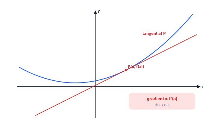
A gradient is also a rate of change. It tells us how much the vertical quantity changes per unit change in the horizontal quantity. Therefore,

$$\frac{dy}{dx}$$

means the instantaneous rate of change of $y$ with respect to $x$.

For example, if $s$ is displacement in metres and $t$ is time in seconds, then

$$\frac{ds}{dt}$$

is velocity in metres per second. A negative derivative means the measured quantity is decreasing at that instant; it does not mean that the magnitude of the rate is negative.

Worked example

Suppose the height of an object is

$$h(t)=t^3-6t^2+12t+1.$$

Then

$$\frac{dh}{dt}=3t^2-12t+12.$$

At $t=3$,

$$\left.\frac{dh}{dt}\right|_{t=3} =27-36+12 =3.$$

The height is increasing at $3$ units per unit time when $t=3$.

The units of a derivative are always

$$\frac{\text{units of the dependent variable}}{\text{units of the independent variable}}.$$

Differentiation from first principles is not required. You should interpret and use derivatives, rather than derive the power rule from a limiting process.

Common trap: $f'(a)$ is a number, while $f'(x)$ is a function. The first is a particular gradient; the second gives gradients throughout the domain.

Two main notations are used for derivatives. If $y=f(x)$, then

$$\frac{dy}{dx}=f'(x).$$

Differentiating again gives the second derivative:

$$\frac{d^2y}{dx^2}=f''(x).$$

The notation is

$$\frac{d^2y}{dx^2},$$

not

$$\left(\frac{dy}{dx}\right)^2.$$

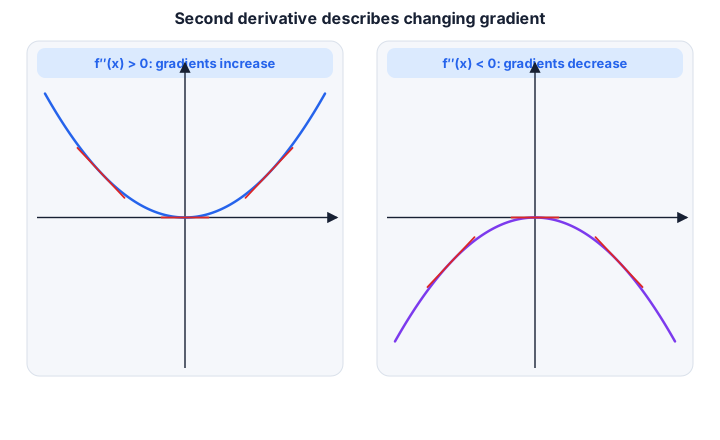
The second derivative measures how the first derivative is changing. Since the first derivative is the gradient function, the second derivative describes how the gradient changes as $x$ changes.

• If $f''(x)>0$, the gradients are increasing.
• If $f''(x)<0$, the gradients are decreasing.
• If $f''(x)=0$, no conclusion can be drawn without further information.

In motion, if $s(t)$ is displacement, then

$$s'(t)$$

is velocity and

$$s''(t)$$

is acceleration.

Worked example

Let

$$f(x)=2x^4-3x^3+5x.$$

Then

$$f'(x)=8x^3-9x^2+5$$

and

$$f''(x)=24x^2-18x.$$

At $x=1$,

$$f'(1)=8-9+5=4,$$

so the tangent gradient is $4$. Also,

$$f''(1)=24-18=6,$$

so the gradient is increasing at that point.

TMUA insight: sometimes only the degree or leading term of a derivative matters. If a question asks for the degree of a differentiated polynomial, identify the highest-power term and check only whether leading terms could cancel. Expanding every term may be unnecessary.

For any rational number $n$, the power rule is

$$\frac{d}{dx}\left(x^n\right)=nx^{n-1},$$

where the real-valued function and its derivative are defined.

Consequently,

$$\frac{d}{dx}\left(ax^n\right)=anx^{n-1},$$

and sums and differences may be differentiated term by term.

Important special cases include

$$\frac{d}{dx}(c)=0,$$

$$\frac{d}{dx}(x)=1,$$

$$\frac{d}{dx}\left(\sqrt{x}\right) =\frac{d}{dx}\left(x^{1/2}\right) =\frac{1}{2}x^{-1/2} =\frac{1}{2\sqrt{x}},$$

and

$$\frac{d}{dx}\left(\frac{1}{x^m}\right) =\frac{d}{dx}\left(x^{-m}\right) =-mx^{-m-1}.$$

Pay attention to domains. For example, $\sqrt{x}$ is real for $x\geq 0$, but its derivative above is defined only for $x>0$. A negative power requires $x\neq 0$.

Within this topic, expressions should usually be expanded, divided through or rewritten using index laws before differentiation. Product, quotient and chain rules are not required.

Worked example: simplifying a quotient

Differentiate

$$y=\frac{(3x+2)^2}{x^2}, \qquad x\neq 0.$$

First expand and divide each term by $x^2$:

$$y=\frac{9x^2+12x+4}{x^2} =9+12x^{-1}+4x^{-2}.$$

Now differentiate term by term:

$$\frac{dy}{dx} =-12x^{-2}-8x^{-3}.$$

An equivalent form is

$$\frac{dy}{dx} =-\frac{12}{x^2}-\frac{8}{x^3}.$$

Worked example: fractional and negative powers

If

$$f(x)=4x^{3/2}-6x^{1/2}+5x^{-2},$$

then

$$f'(x) =6x^{1/2}-3x^{-1/2}-10x^{-3}.$$

Common traps

• Do not reduce the exponent without multiplying by the original exponent.
• Do not treat $(3x+2)^2$ as $9x^2+4$; the middle term is essential.
• Do not use a quotient rule when elementary algebra turns the expression into a sum of powers.
• Preserve the domain restrictions created by denominators and roots.

For a curve $y=f(x)$, the tangent gradient at $x=a$ is

$$m_{\text{tangent}}=f'(a).$$

The point of contact is

$$(a,f(a)).$$

Using point-gradient form, the tangent is

$$y-f(a)=f'(a)(x-a).$$

A normal is perpendicular to the tangent. If the tangent gradient is non-zero, then

$$m_{\text{normal}}=-\frac{1}{f'(a)},$$

so the normal is

$$y-f(a)=-\frac{1}{f'(a)}(x-a).$$

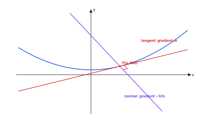
If $f'(a)=0$, the tangent is horizontal and the normal is the vertical line

$$x=a.$$

Do not attempt to calculate $-1/0$.

Worked example

Find the tangent and normal to

$$y=x^3-2x$$

at $x=1$.

The point on the curve is

$$(1,1^3-2)=(1,-1).$$

Differentiate:

$$\frac{dy}{dx}=3x^2-2.$$

At $x=1$, the tangent gradient is

$$3(1)^2-2=1.$$

Therefore the tangent is

$$y+1=x-1,$$

so

$$y=x-2.$$

The normal gradient is $-1$, giving

$$y+1=-(x-1),$$

so

$$y=-x.$$

For two curves to touch tangentially at the same point, both conditions are needed:

$$f(a)=g(a)$$

and

$$f'(a)=g'(a).$$

Meeting at the same point alone does not prove tangency.

Efficient method: for the shortest distance from a curve to a fixed line, the joining segment is perpendicular to both at the closest point. Therefore, the tangent to the curve at that point is parallel to the fixed line. Equating their gradients can locate the relevant point before any distance calculation.

A stationary point occurs where the tangent is horizontal:

$$f'(x)=0.$$

Solving this equation gives the possible $x$-coordinates. Substitute each value into $f(x)$ to obtain the full coordinates.

A stationary point is not automatically a maximum or minimum. It must be classified.

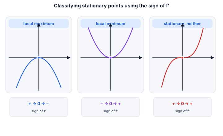
First-derivative sign test

Consider the sign of $f'(x)$ immediately on either side of the stationary value.

• Positive then negative: local maximum.
• Negative then positive: local minimum.
• No sign change: neither a maximum nor a minimum.

Second-derivative test

At a stationary point $x=a$:

$$f'(a)=0 \quad\text{and}\quad f''(a)>0 \implies \text{local minimum},$$

while

$$f'(a)=0 \quad\text{and}\quad f''(a)<0 \implies \text{local maximum}.$$

If

$$f''(a)=0,$$

the test is inconclusive. For example, at $x=0$:

• $y=x^4$ has a local minimum;
• $y=-x^4$ has a local maximum;
• $y=x^3$ has neither.

All three have first and second derivatives equal to zero at the origin.

Worked example

Find and classify the stationary points of

$$f(x)=2x^3-3x^2-12x+6.$$

Differentiate:

$$f'(x)=6x^2-6x-12 =6(x-2)(x+1).$$

Hence stationary points occur at

$$x=-1 \quad\text{and}\quad x=2.$$

Their coordinates are

$$f(-1)=13$$

and

$$f(2)=-14.$$

Now

$$f''(x)=12x-6.$$

Therefore,

$$f''(-1)=-18<0,$$

so $(-1,13)$ is a local maximum, and

$$f''(2)=18>0,$$

so $(2,-14)$ is a local minimum.

TMUA shortcuts and traps

• For a cubic, $f'(x)$ is quadratic. Its discriminant can quickly reveal whether there are two, one or no stationary $x$-values.
• Use the known end behaviour of a polynomial to support a sketch and classification.
• A local maximum need not be the greatest value over the whole domain, and a local minimum need not be the least.
• Always give both coordinates when a question asks for a stationary point, not just the solution of $f'(x)=0$.
• Never claim that $f''(a)=0$ proves a point of inflection.

A function is strictly increasing on an interval when larger inputs always produce larger outputs. It is strictly decreasing when larger inputs always produce smaller outputs.

For the differentiable functions considered here:

$$f'(x)>0$$

throughout an interval is sufficient to show that $f$ is strictly increasing there, while

$$f'(x)<0$$

throughout an interval is sufficient to show that $f$ is strictly decreasing there.

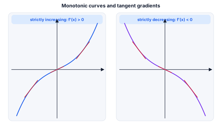
To find intervals of increase and decrease:

1. Calculate $f'(x)$.
2. Find the critical values where $f'(x)=0$ or is undefined.
3. Determine the sign of $f'(x)$ on each interval.
4. State the intervals using inequalities.

Worked example

Let

$$f(x)=x^3-3x.$$

Then

$$f'(x)=3x^2-3 =3(x-1)(x+1).$$

The derivative is positive when

$$x<-1 \quad\text{or}\quad x>1,$$

and negative when

$$-1<x<1.$$

Therefore $f$ is strictly increasing on

$$(-\infty,-1) \quad\text{and}\quad (1,\infty),$$

and strictly decreasing on

$$(-1,1).$$

Be careful with the logic. The implication

$$f'(x)>0 \implies f \text{ is strictly increasing}$$

does not reverse in every case. For example, $f(x)=x^3$ is strictly increasing on the real numbers, but

$$f'(0)=0.$$

Thus a strictly increasing function need not have a strictly positive derivative at every single point.

Efficient sign analysis: when $f'(x)$ is factorised, use the signs of its factors rather than substituting many numerical values. Check only one value in each interval if the sign is not immediately clear.

A point of inflection is a point where the curve changes the direction in which it bends: from bending upwards to bending downwards, or vice versa.

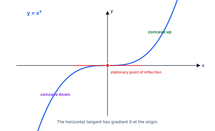
A point of inflection need not be stationary. For example,

$$y=x^3+x$$

changes its bending at the origin, but

$$\frac{dy}{dx}=3x^2+1,$$

so the gradient there is $1$, not $0$.

For simple polynomials, the sign of the second derivative can help describe the change in bending:

• $f''(x)>0$ corresponds to increasing gradients;
• $f''(x)<0$ corresponds to decreasing gradients.

A change of sign in $f''(x)$ is consistent with a point of inflection. However,

$$f''(a)=0$$

by itself is not enough. For instance, $y=x^4$ has $f''(0)=0$ but no change in bending at the origin.

The examinable requirement is qualitative. You should recognise the possible presence of an inflection when interpreting or sketching a simple polynomial, but you are not expected to carry out a technical classification of inflection points.