Graphs of Functions

A graph is a visual record of how the output of a function changes as its input changes. A useful sketch is not a collection of guessed points: it should show the features that control the whole shape.

Before drawing a graph, identify as many of the following as are relevant:

• the domain and range;
• the intercepts with the coordinate axes;
• any symmetry;
• stationary points;
• asymptotes or excluded values;
• whether the function is increasing or decreasing;
• the behaviour for large positive and negative values of $x$.

A sketch does not need to be drawn to scale, but every marked intercept, turning point and asymptote must be consistent with the equation.

Straight lines

The graph of

$$y=mx+c$$

is a straight line with gradient $m$ and $y$-intercept $c$. Two accurately placed points are enough to determine it. The effects of $m$ and $c$ are developed in a later section.

Quadratics

A quadratic has the form

$$y=ax^2+bx+c, \qquad a\ne 0.$$

Its graph is a parabola. It opens upwards when $a>0$ and downwards when $a<0$. Its axis of symmetry passes through its maximum or minimum point.

The discriminant

$$\Delta=b^2-4ac$$

determines how the graph meets the $x$-axis:

• $\Delta>0$: two distinct $x$-intercepts;
• $\Delta=0$: one repeated intercept, where the graph touches the axis;
• $\Delta<0$: no real $x$-intercepts.

Writing a quadratic in completed-square form makes its vertex and axis of symmetry immediately visible.

Cubics and higher-degree polynomials

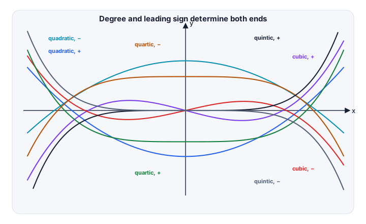
The highest-power term controls the end behaviour of a polynomial. For

$$p(x)=a_nx^n+\cdots+a_1x+a_0, \qquad a_n\ne 0,$$

the term $a_nx^n$ dominates when $|x|$ is large.

For even $n$, the two ends of the graph point in the same vertical direction:

• if $a_n>0$, both ends rise;
• if $a_n<0$, both ends fall.

For odd $n$, the ends point in opposite directions:

• if $a_n>0$, the graph falls to the left and rises to the right;
• if $a_n<0$, the graph rises to the left and falls to the right.

A cubic can be always increasing or always decreasing, or it can have a local maximum and a local minimum. It can have one, two or three distinct real roots; two distinct roots occur when one is repeated.

Trigonometric functions

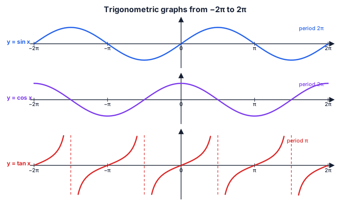
Angles are normally measured in radians.

For $y=\sin x$:

• the range is $[-1,1]$;
• the period is $2\pi$;
• the graph passes through $(0,0)$;
• zeros occur at $x=n\pi$, where $n$ is an integer.

For $y=\cos x$:

• the range is $[-1,1]$;
• the period is $2\pi$;
• the graph passes through $(0,1)$;
• zeros occur at $x=\frac{\pi}{2}+n\pi$.

For $y=\tan x$:

• the range is all real numbers;
• the period is $\pi$;
• zeros occur at $x=n\pi$;
• vertical asymptotes occur at

$$x=\frac{\pi}{2}+n\pi.$$

A tangent curve must not be drawn through one of its vertical asymptotes.

Exponential functions

For

$$y=a^x, \qquad a>0,\quad a\ne 1,$$

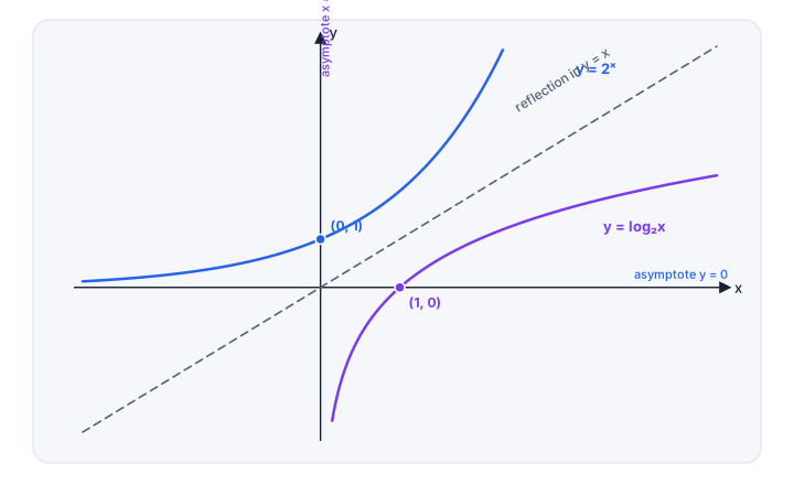
the graph always passes through $(0,1)$ and always lies above the $x$-axis. The line $y=0$ is a horizontal asymptote.

• If $a>1$, the function is increasing.
• If $0<a<1$, the function is decreasing.

There is no $x$-intercept because $a^x>0$ for every real $x$.

Logarithmic functions

The graph of

$$y=\log_a x, \qquad a>0,\quad a\ne 1,$$

is the inverse of $y=a^x$. Its domain is $x>0$, it passes through $(1,0)$, and $x=0$ is a vertical asymptote.

• If $a>1$, the function is increasing.
• If $0<a<1$, the function is decreasing.

The exponential and logarithmic graphs with the same base are reflections of one another in the line $y=x$.

Square-root functions

The parent graph

$$y=\sqrt{x}$$

has domain $x\ge 0$ and range $y\ge 0$. It begins at $(0,0)$, increases, and becomes less steep as $x$ increases. A translated square-root graph begins where the expression inside the square root first becomes zero.

The modulus function

The modulus of a real number is its distance from zero:

$$|x|= \begin{cases} x, & x\ge 0,\\ -x, & x<0. \end{cases}$$

Therefore $y=|x|$ is a V-shaped graph with vertex at the origin.

More generally,

$$y=|f(x)|$$

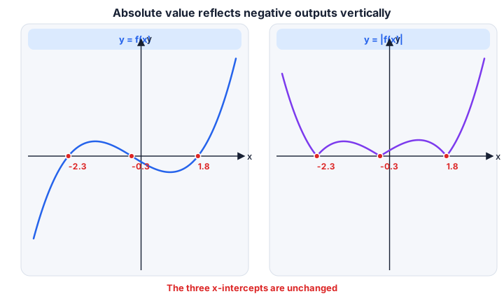
leaves every part of $y=f(x)$ on or above the $x$-axis unchanged and reflects every part below the $x$-axis in that axis. The $x$-intercepts stay in the same places.

Common mistake: $y=|f(x)|$ does not reflect the graph in the $y$-axis. It changes output values, so the reflection is vertical.

A fast TMUA sketch should prioritise exact structural features over decorative accuracy. Mark known coordinates and asymptotes first, then join them with a curve whose direction and end behaviour agree with the function.

Suppose the graph of $y=f(x)$ is known. Transformations change either the outputs of $f$, the inputs of $f$, or both.

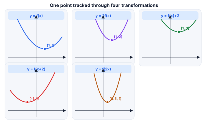
A reliable way to avoid sign and scale errors is to track how a general point $(x,y)$ on the original graph moves.

The transformation $y=af(x)$

Every output is multiplied by $a$:

$$(x,y)\longmapsto (x,ay).$$

• If $|a|>1$, the graph is stretched parallel to the $y$-axis by scale factor $|a|$.
• If $0<|a|<1$, it is compressed parallel to the $y$-axis.
• If $a<0$, it is also reflected in the $x$-axis.

The $x$-intercepts are unchanged, because multiplying an output of zero still gives zero.

The transformation $y=f(x)+a$

Every output increases by $a$:

$$(x,y)\longmapsto (x,y+a).$$

This is a translation by the vector

$$\begin{pmatrix} 0\\ a \end{pmatrix}.$$

A positive $a$ moves the graph up; a negative $a$ moves it down.

The transformation $y=f(x+a)$

The graph is translated horizontally in the direction opposite to the sign written inside the function:

$$(x,y)\longmapsto (x-a,y).$$

Thus $f(x+3)$ moves the graph three units left, while $f(x-3)$ moves it three units right.

This reversal happens because a point that originally required input $x$ now requires the new input $x-a$, since

$$(x-a)+a=x.$$

The transformation $y=f(ax)$

The input is multiplied by $a$. A point moves according to

$$(x,y)\longmapsto \left(\frac{x}{a},y\right).$$

• The horizontal scale factor is $\frac{1}{|a|}$.
• If $a<0$, the graph is also reflected in the $y$-axis.

The reciprocal scale factor is a frequent source of errors. For example, $y=f(4x)$ is four times narrower, not four times wider.

Compositions of transformations

Several transformations may be combined. Rather than relying on a memorised order, rewrite the expression clearly or map a general point.

For example, consider

$$y=-2f\bigl(3(x-1)\bigr)+4.$$

If $(u,v)$ lies on $y=f(x)$, then the new input must satisfy

$$3(x-1)=u,$$

so

$$x=1+\frac{u}{3}.$$

The output becomes

$$-2v+4.$$

Therefore the complete point mapping is

$$(u,v)\longmapsto \left(1+\frac{u}{3},\, -2v+4\right).$$

This shows a horizontal compression by scale factor $\frac13$, a shift right by $1$, a reflection in the $x$-axis, a vertical stretch by scale factor $2$, and a shift up by $4$.

Efficient TMUA method: transform important points rather than trying to redraw the entire curve after every step. Intercepts, endpoints, vertices and asymptote-defining points usually determine the answer.

Function composition

The notation

$$f(g(x))$$

means that $g$ acts first and its output is then used as the input of $f$. In general,

$$f(g(x))\ne g(f(x)).$$

For example, let

$$f(x)=x^2+1, \qquad g(x)=2x-3.$$

Then

$$f(g(x))=(2x-3)^2+1,$$

whereas

$$g(f(x))=2(x^2+1)-3=2x^2-1.$$

The domain of a composition must also be checked. An input $x$ is allowed in $f(g(x))$ only when $x$ is in the domain of $g$ and $g(x)$ lies in the domain of $f$.

For instance, if $f(x)=\sqrt{x}$, then $f(g(x))$ requires

$$g(x)\ge 0.$$

Common mistake: in $f(g(x))$, do not replace $x$ in $g$ by $f(x)$. Read compositions from the inside out.

For

$$y=mx+c,$$

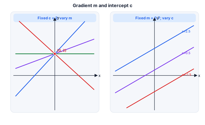
the parameter $m$ is the gradient and $c$ is the $y$-intercept.

The gradient measures the change in $y$ for each unit increase in $x$:

$$m=\frac{\text{change in }y}{\text{change in }x}.$$

• If $m>0$, the line rises from left to right.
• If $m<0$, the line falls from left to right.
• If $m=0$, the line is horizontal.
• A larger value of $|m|$ gives a steeper line.

Changing $m$ while keeping $c$ fixed rotates the line about the fixed point $(0,c)$. Changing $c$ while keeping $m$ fixed translates the line vertically, producing parallel lines.

The intercepts are found algebraically:

• $y$-intercept: set $x=0$, giving $(0,c)$;
• $x$-intercept: set $y=0$, giving

$$x=-\frac{c}{m}, \qquad m\ne 0.$$

Worked example

Sketch the main features of

$$y=-3x+6.$$

The gradient is $-3$, so the line falls steeply from left to right. Its $y$-intercept is

$$(0,6).$$

For the $x$-intercept,

$$0=-3x+6,$$

so $x=2$. The line therefore passes through $(0,6)$ and $(2,0)$.

When comparing several straight-line graphs in a TMUA question, calculate only what distinguishes the options. The sign of the gradient, the $y$-intercept and one additional point are often enough.

The form

$$y=a(x+b)^2+c, \qquad a\ne 0,$$

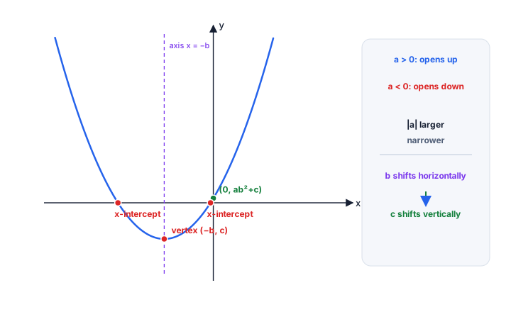
shows the geometry of a quadratic directly.

Because $(x+b)^2\ge 0$, the vertex occurs when

$$x+b=0.$$

Therefore the vertex is

$$(-b,c),$$

and the axis of symmetry is

$$x=-b.$$

The parameter $a$ controls the orientation and vertical scale:

• $a>0$: the graph opens upwards and the vertex is a minimum;
• $a<0$: the graph opens downwards and the vertex is a maximum;
• larger $|a|$: the parabola is narrower;
• smaller non-zero $|a|$: the parabola is wider.

The parameter $b$ controls horizontal position, with the direction opposite to its sign. The parameter $c$ controls vertical position.

The range is

$$y\ge c \quad \text{if } a>0,$$

and

$$y\le c \quad \text{if } a<0.$$

The $y$-intercept is found by setting $x=0$:

$$y=ab^2+c.$$

For the $x$-intercepts, solve

$$a(x+b)^2+c=0.$$

This gives

$$(x+b)^2=-\frac{c}{a}.$$

Hence:

• if $-\frac{c}{a}>0$, there are two distinct roots;
• if $-\frac{c}{a}=0$, there is one repeated root at the vertex;
• if $-\frac{c}{a}<0$, there are no real roots.

Worked example

Consider

$$y=-2(x-3)^2+8.$$

Here $a=-2$, $b=-3$ and $c=8$. Therefore:

• the vertex is $(3,8)$;
• the axis of symmetry is $x=3$;
• the graph opens downwards;
• the maximum value is $8$.

The $x$-intercepts satisfy

$$-2(x-3)^2+8=0.$$

Therefore

$$(x-3)^2=4,$$

so

$$x=1 \quad \text{or} \quad x=5.$$

The $y$-intercept is

$$-2(0-3)^2+8=-10.$$

These features determine the sketch without a table of values.

A quadratic in general form can be converted into this form. For

$$y=Ax^2+Bx+C, \qquad A\ne 0,$$

completing the square gives

$$y=A\left(x+\frac{B}{2A}\right)^2 +C-\frac{B^2}{4A}.$$

Therefore its vertex is

$$\left( -\frac{B}{2A}, \, C-\frac{B^2}{4A} \right).$$

Common mistake: in $a(x+b)^2+c$, the horizontal coordinate of the vertex is $-b$, not $b$.

Differentiation links an equation to the gradient of its graph. If

$$y=f(x),$$

then $f'(x)$ gives the gradient at each point where the derivative exists.

The sign of $f'(x)$ determines whether the graph rises or falls:

$$f'(x)>0 \quad\Longrightarrow\quad f \text{ is increasing},$$

$$f'(x)<0 \quad\Longrightarrow\quad f \text{ is decreasing}.$$

A stationary point occurs where

$$f'(x)=0.$$

To classify a stationary point within the required scope, examine the sign of $f'(x)$ on either side:

• positive then negative: local maximum;
• negative then positive: local minimum.

Solving $f'(x)=0$ only identifies candidates. A sign check is needed to determine how the graph behaves.

A systematic sketching method

1. Find the domain and any asymptotes.
2. Find the coordinate-axis intercepts where possible.
3. Determine the end behaviour.
4. Differentiate and solve $f'(x)=0$.
5. Use a sign chart for $f'(x)$.
6. Calculate the coordinates of the stationary points.
7. Join the information with a smooth curve consistent with all features.

Worked example

Let

$$f(x)=x^3-3x^2-9x+5.$$

Differentiate:

$$f'(x)=3x^2-6x-9 =3(x+1)(x-3).$$

The stationary values of $x$ are

$$x=-1 \quad\text{and}\quad x=3.$$

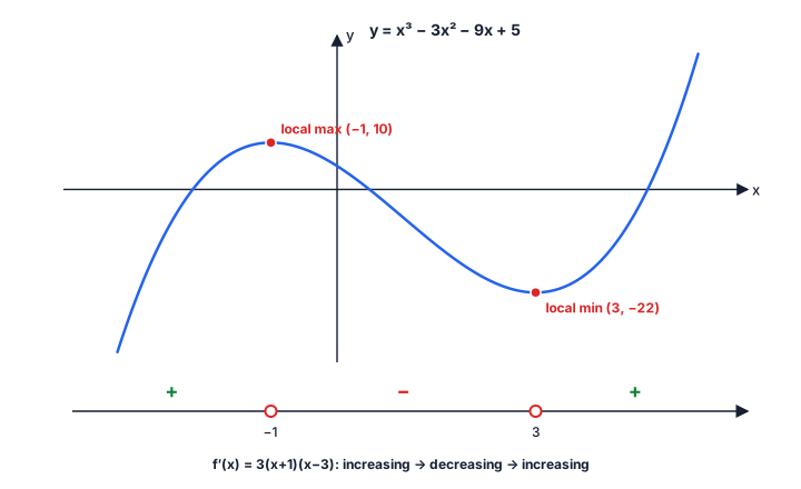
The sign of $f'(x)$ is:

• positive for $x<-1$;
• negative for $-1<x<3$;
• positive for $x>3$.

Therefore the graph increases, then decreases, then increases. It has a local maximum at $x=-1$ and a local minimum at $x=3$.

Their coordinates are

$$f(-1)=10,$$

and

$$f(3)=-22.$$

So the stationary points are

$$(-1,10) \quad\text{and}\quad (3,-22).$$

The leading term is $x^3$, so the graph falls to the left and rises to the right.

Efficient TMUA method: keep the derivative factorised. Its factors reveal where the sign can change. For a simple linear factor, the sign changes when its root is crossed; for a repeated factor, it may not. Test one value in each interval only when the sign is not immediately clear.

Common mistake: a stationary point is not automatically a maximum or minimum. The derivative must change sign in the appropriate way.

The graph of $y=f(x)$ meets the $y$-axis when $x=0$. Its $y$-intercept is therefore

$$(0,f(0)).$$

It meets the $x$-axis where $y=0$, so its $x$-intercepts correspond exactly to the real solutions of

$$f(x)=0.$$

Useful algebraic methods include:

• taking out a common factor;
• factorising quadratics;
• using identities such as the difference of two squares;
• completing the square;
• using the quadratic formula or discriminant;
• making a substitution when the expression is quadratic in another quantity.

Worked example

For

$$p(x)=x^4-5x^2+4,$$

treat the expression as a quadratic in $x^2$:

$$p(x)=(x^2-1)(x^2-4).$$

Then

$$p(x)=(x-1)(x+1)(x-2)(x+2).$$

The four real roots are

$$x=-2,-1,1,2.$$

The graph therefore crosses the $x$-axis at four distinct points.

Degree and possible numbers of roots

A non-zero polynomial of degree $n$ has at most $n$ distinct real roots. If it had more, it would have more linear factors than its degree allows.

An odd-degree polynomial must have at least one real root because its two ends point in opposite vertical directions and a polynomial graph is continuous. An even-degree polynomial can have no real roots.

Thus:

• a quadratic can have $0$, $1$ or $2$ distinct real roots;
• a cubic can have $1$, $2$ or $3$ distinct real roots;
• a degree-$n$ polynomial can never have more than $n$ distinct real roots.

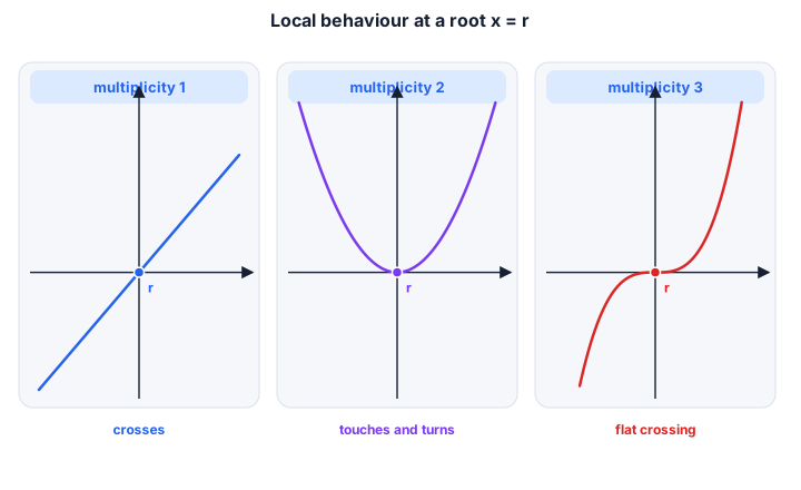
A repeated factor changes how the graph meets the axis. If

$$f(x)=(x-r)^kq(x), \qquad q(r)\ne 0,$$

then $r$ is a root of multiplicity $k$.

• For odd $k$, the graph crosses the axis at $x=r$.
• For even $k$, the graph touches the axis and turns back.

Counting roots without solving them

Sometimes the roots cannot be found exactly, but their number can still be determined from:

• end behaviour;
• stationary points;
• the signs of the function at selected values;
• known transformations;
• the discriminant when a quadratic is involved.

For example, consider

$$y=x^2-4x+k.$$

Its discriminant is

$$\Delta=(-4)^2-4(1)(k)=16-4k.$$

Therefore:

• $k<4$: two real roots;
• $k=4$: one repeated real root;
• $k>4$: no real roots.

Geometrically, varying $k$ translates the parabola vertically.

Common mistakes:

• solving $f(x)=0$ but forgetting to convert the roots into points $(x,0)$ when coordinates are requested;
• assuming that a degree-$n$ polynomial must have $n$ real roots;
• cancelling a factor containing $x$, which may discard a valid zero root.

A point lies on both

$$y=f(x)$$

and

$$y=g(x)$$

exactly when its coordinates satisfy both equations. At an intersection,

$$f(x)=g(x).$$

Therefore the $x$-coordinates of the intersections are the real solutions of

$$f(x)-g(x)=0.$$

After finding an $x$-value, substitute it into either original equation to find the corresponding $y$-value.

This gives the geometric meaning of simultaneous equations: each solution pair is an intersection point of the corresponding graphs.

Number and type of intersections

• No real solution means the graphs do not meet.
• One solution means they meet once; this may be a crossing or a tangency.
• Several solutions mean several intersection points.
• If the two equations describe the same graph, there are infinitely many common points.

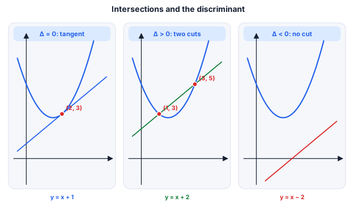
For a line and a quadratic, substitution produces a quadratic equation. Its discriminant determines whether there are zero, one or two intersections.

Worked example

Find the intersections of

$$y=x+1$$

and

$$y=x^2-3x+5.$$

Equate the two expressions for $y$:

$$x+1=x^2-3x+5.$$

Rearranging,

$$x^2-4x+4=0,$$

so

$$(x-2)^2=0.$$

There is one repeated solution, $x=2$. Substituting into $y=x+1$ gives

$$y=3.$$

The graphs meet at

$$(2,3).$$

Because the resulting equation has a repeated root, the line is tangent to the parabola there.

Equations can often be interpreted as intersections with familiar graphs:

• $f(x)=0$: intersections of $y=f(x)$ with the $x$-axis;
• $f(x)=k$: intersections of $y=f(x)$ with the horizontal line $y=k$;
• $f(x)=mx+c$: intersections of $y=f(x)$ with a straight line.

This interpretation is especially useful when a question asks only for the number of solutions. A sketch, monotonicity argument or discriminant calculation may be much faster than attempting exact algebra.

If $f$ and $g$ are polynomials, the number of intersections is controlled by the degree of

$$f(x)-g(x).$$

For example, two distinct quadratics usually give a quadratic equation after subtraction, so they can have at most two intersections. If their quadratic terms cancel, the resulting equation may be linear or constant. If every term cancels, the graphs are identical.

Efficient TMUA method: first decide what kind of equation $f(x)=g(x)$ produces. Factorisation, the discriminant, or a graph-shape argument may give the number of intersections without finding every coordinate.

Common mistake: the intersections of $y=f(x)$ and $y=g(x)$ are found from $f(x)=g(x)$, not from solving $f(x)=0$ and $g(x)=0$ separately.